SHAP Values and Model Explainability

Imagine you’ve built a powerful, and complex machine learning model that predicts some outcome $y$. Although it performs very well, when you present it to the relevant stakeholders, they ask you why the model predicts $y_1$ instead of $y_2$. What “drives” the outcome?

This is a difficult question to answer, because the complex model you’ve built isn’t as interpretable as linear regression would be. You can’t easily determine how changing one input variable affects the prediction, or quantify how each feature contributes to the final output. For example, you can’t confidently say weather a input variable $x_1$ has a positive effect on the outcome $\hat{y}$.

It turns out there exists a framework that tries to answer exactly this: How much does each feature contribute towards the predictions?

The framework is called SHAP, which stands for SHapley Additive exPlanations (Lundberg and Lee). It’s a general framework for “explaining” machine learning models, which is model-agnostic, meaning it works for all types of models, from tree-based models like XGBoost and CatBoost to neural networks.

As the name suggests, SHAP is based on an old game-theoretic concept called Shapley values.

Shapley values, and by extension SHAP values, are a way to fairly distribute the total gains (or “payout”) of a collaborative game to the participants of the game.

We can relate this to machine learning models by thinking of a model as a game played by the input variables. The features work together to obtain a model output $\hat{y}$. Thus, SHAP values are an application of Shapley values to machine learning model explanations. The framework also consists of approximation methods for estimating the values. These are maintained in the shap library.

As an example, I have built a machine learning model that predicts if a climber will end up on the podium at IFSC climbing competitions (the Boulder and Boulder&Lead disciplines). Hence, it’s a classifier that predicts a binary outcome is_on_podium. It’s neither powerful nor complex, but perfect for illustrative purposes. I chose to use an XGBoost classifier with one-hot-encoding applied to the categorical features (all the code is available here).

Here is a plot of the xgboost feature importances (which are not related to SHAP):

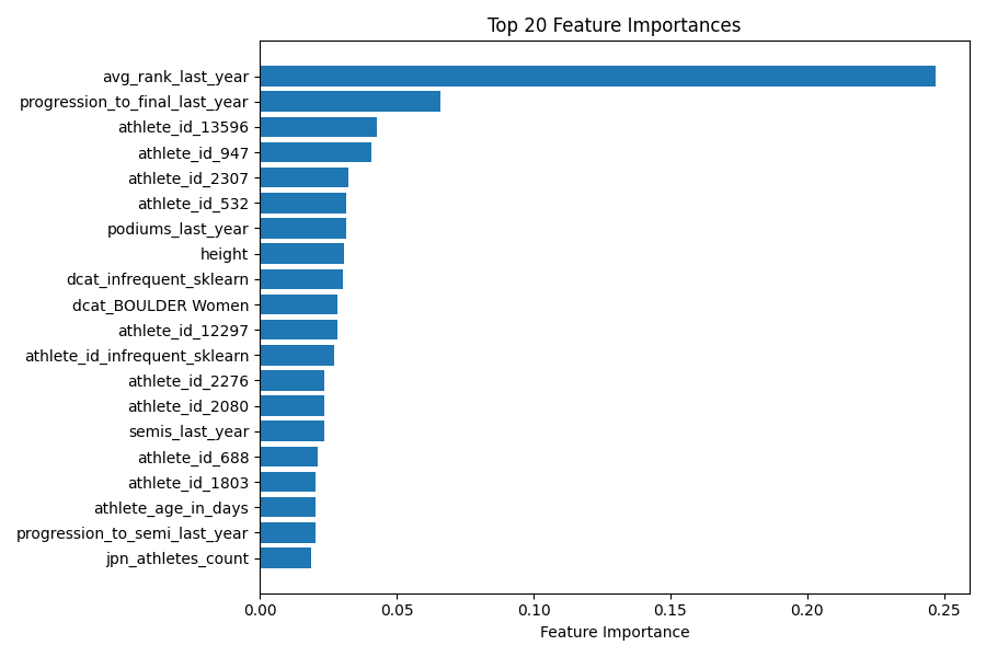
The most important feature is avg_rank_last_year. This aligns with expectations. It’s usually the athletes who performed well previously, who also perform well later. Same logic applies to progression_to_final_last_year. The feature height is also in the top 20 most important features, which is less intuitive. “Height” is often discussed at climbing competitions, because most climbers aren’t tall, even though the casual viewer might expect height to be an advantage. But remember, high feature importance says nothing about whether shorter or taller climbers are at an advantage.

Feature importances measure how much a feature contributes to improving the model’s predictive performance, typically by reducing prediction error. SHAP values, on the other hand, measure how much a feature contributes to the model’s output. While feature importances are global (one value for each feature across the entire dataset), SHAP values are both local and global. We can compute the SHAP values of input features for a single observation (local explanation) or average them out over all observations (to obtain a global explanation).

Here is a plot of the top 9 features with the highest mean absolute SHAP values:

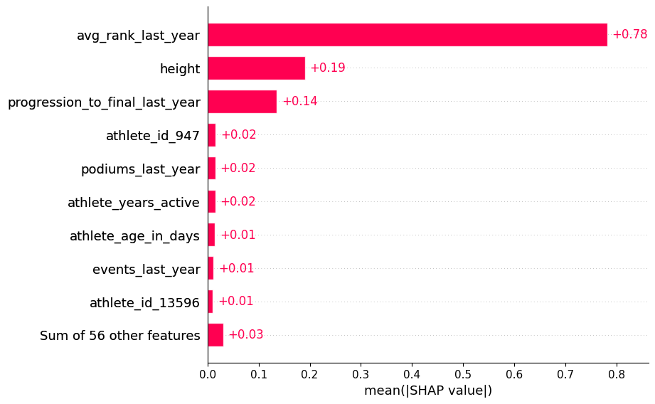
We notice some similarities with the feature importances, e.g., avg_rank_last_year and progression_to_final_last_year are at the top. However, height also has a relatively high mean absolute SHAP value. Let’s dig deeper into this with another plot:

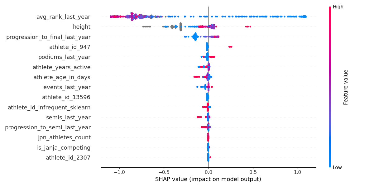
This plot shows the SHAP value for each observation, where the dots are colored according to their observed value. So for avg_rank_last_year, all the blue dots indicate observations with a low value, i.e., where an athlete has performed well and ranked at the top. It seems our assumption was correct; ranking high at previous competitions generally contributes positively to the model’s output.

height is different. There are clusters of red (i.e., tall climbers) with both positive and negative constributions. Same for blue (and remember, if you mix blue and red, you get purple). The grey dots are observations with a missing value for height.

Finally, let’s look at a waterfall plot of the SHAP values for an individual observation. This is for the Japanese athlete Sorato Anraku at the Boulder World Cup in Bern 2025:

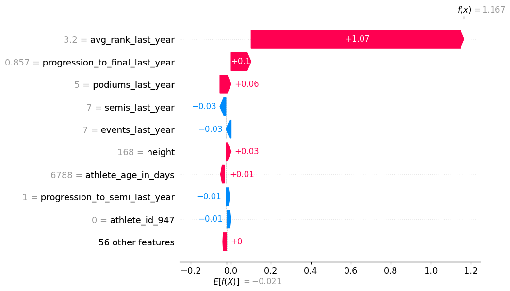
This plot is great for illustrating some of the details regarding SHAP values. First off, we can see that the model’s output for this observation is $f(x) = 1.167$.

Since we are predicting a binary outcome, we typically expect the final model prediction to be a probability in the range [0,1]. However, SHAP works with the raw model output (in this case, log-odds), not the transformed probability. We can obtain the model output probability from the raw model output by applying the sigmoid function, defined as $\sigma(x) = \tfrac{1}{1 + e^{-x}}$. Hence, the model output is

\[\hat{y}_\text{sorato, bern} =\sigma(1.167) = \frac{1}{1 + e^{-1.167}} = 0.76.\]

So with the usual threshold of $0.5$, the model predicts Sorato will end up on the podium (spoiler alert: he does. He ranks third.)

A defining feature of SHAP values is that the SHAP values for all features of a single observation sum up to the difference between the model output and the expected output (a property called local additivity).

The expected raw model output across the background dataset is $E[f(X)]=−0.021$, which corresponds to a probability of $\sigma(−0.021)≈0.49$. This is the baseline SHAP uses as a reference point, though due to imbalances in the data, it’s not necessarily equal to the overall average prediction probability.

As mentioned earlier, the SHAP framework also consists of methods for estimating the values. I won’t touch upon it here, but computing SHAP values are computationally expensive, so it’s usually only done on a small sample of the data (often just 1000 rows), and even then, it’s still intensive. The expected raw model output is also computed from this small sample of the data.

So to recap:

• SHAP values are an application of Shapley values from game theory to machine learning model explanations.
• SHAP is model-agnostic, meaning it can be applied to all types of models, including tree-based models and neural networks.
• SHAP values measure the contribution of a feature to the difference between the model’s output and its expected model output.
• Because exact SHAP calculations are expensive, the SHAP library includes efficient approximation methods.
• Bonus: SHAP values for a binary classifer are in log-odds space and not in probability space.

Finally, be aware that SHAP values explain model predictions, not causal effects. A large SHAP value means the feature strongly influenced the prediction for that model and that dataset, not that it’s universally important. In addition, while SHAP is very popular, it’s not without its critics (see, for example, “SHAP is the Blockchain of xAI”), so have some caution before relying on SHAP as the sole source of model explainability.

---

References

1. Lundberg, Scott M., and Su-In Lee. “A Unified Approach to Interpreting Model Predictions.” CoRR, vol. abs/1705.07874, 2017, http://arxiv.org/abs/1705.07874.