One-dimensional smoothing methods: LOESS and LOWESS

19 June 2025

When data is noisy or the underlying relationship is not well captured by a simple curve, we can turn to smoothing methods. Locally estimated/weighted scatterplot smoothing (LOESS or LOWESS for short) provide a way to estimate flexible, smooth curves by fitting simple models to local neighborhoods of the data. This allows us to uncover patterns without assuming a fixed global shape.

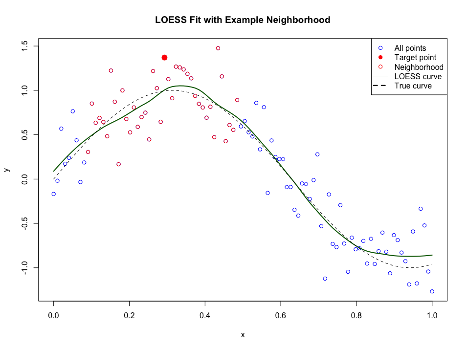
The plot shows 100 data points $(x_i, y_i)$ generated from the dashed curve $Y = \sin(5X) + \epsilon$, $X \sim U(0,1)$, $\epsilon \sim \mathcal{N}(0, 0.3)$. The green curve is the result of a loess fit with local polynomials of degree 2 and $\text{span} = 0.3$. The filled red dot is an arbitrary target point and the red circles are its neighborhood. This plot was inspired by Figure 6.1 of (Hastie et al., p.192).

How it works

For each target point $x_0$, take the set of $k$ nearest neighbors measured in absolute distance. We call this set a neighborhood and denote it by $N_k(x_0)$. Then fit a simple model using only the points in this neighborhood with weighted least squares regression, where the fit is either linear or polynomial. Usually, LOWESS refers to the case where the fit is linear, while LOESS is the more general case where we fit local polynomials of any degree.

Weights are assigned to the points by the tri-cube function:

\[w(x_i, x_0) := \left( 1- \frac{ | x_i - x_0 | }{d_{max}(x_0)}^3 \right)^3 \quad \text{for } |x_i - x_0| \leq d_{max}(x_0),\]

where $d_{max}(x_0)$ is the distance from $x_0$ to the furthest point in the neighborhood, that is:

\[d_{max}(x_0) = \max_{x \in N_k(x_0)} | x - x_0 |.\]

The tri-cube function assigns weights that decrease smoothly the further away from the target point $x_0$ we get, and this ensures the fitted function is continuous. This is a step-up compared to a simple moving average, for example.

Even though we fit a model to the entire neighborhood, we only use it to evaluate the fit at $x_0$. For all other points, we perform the steps described above again. For the first $k/2$ points, the neighborhood will be the same, but the local fits will not, since the weight assigned to each point will be different.

How smooth the complete fit it is, is generally controlled by the size $k$ of the neighborhoods and the degree of the polynomials we fit. If the size is large, then the fit will be smoother. If we increase the degree of the polynomials, the fit will become more wiggly. Thus, both present a bias-variance trade-off.

In practice, the size of the neighborhood is often expressed as a span $k/N$, where $N$ is the total number of observations.

Beyond single-variable smoothing

While LOESS works great for a single predictor, real-world data often involve more predictors and more complex relationships. In such cases, we could, for example, fit generalized additive models (GAMs), where LOESS applied to one predictor is just one of many terms in the model. This is implemented in the R package gam, but if you want to use another package (such as mgcv) or an entirely different language (e.g. python or julia), LOESS might not be implemented as a smoother. But there are other smoothing options in these cases; such as splines, which seems to be the default in most cases. However, the aim remains the same.

References

Hastie, Trevor, et al. The Elements of Statistical Learning: Data Mining, Inference, and Prediction. 2nd ed, Springer, 2009.

← Back to Blog