Bayesian Inference

In Bayesian inference, we treat parameters as random variables, meaning they have a probability distribution. This is in contrast to classical (frequentist) inference where model parameters are considered fixed. Bayesian inference seeks to make probability statements about parameters conditional on the observed data. It amounts to deriving a posterior probability $p(\theta \mid y)$ as a consequence of a prior probability $p(\theta)$ and a likelihood $p(y \mid \theta)$, where $\theta$ denotes a model parameter, and $y$ is the observed data. The posterior probability is computed according to Bayes’ Theorem:

\[\overbrace{p(\theta \mid y)}^{\text{posterior}} = \frac{\overbrace{p(y\mid \theta)}^{\text{likelihood}}\overbrace{p(\theta)}^{\text{prior}}}{\underbrace{p(y)}_{\text{evidence}}}.\tag{1}\]

The evidence $p(y)$ is also known as the marginal likelihood and can be written as

\[p(y) = \int p(y\mid \theta)p(\theta)d\theta.\tag{2}\]

It represents the probability of seeing the observed data over all possible values of $\theta$. This is often very difficult to compute, which is why Bayesian inference relies on [[conjugate priors]], which are algebraically convenient, or computational approximations (e.g. using MCMC methods or Variational Inference).

A discrete example

Let’s consider a sequence of $n$ Bernoulli trials. We aim to estimate the unknown probability of success $\theta$. A natural model for data that arise from such a sequence is the binomial distribution, with a probability mass function of the form

\[p(y\mid \theta) = \binom{n}{y} \theta^y(1-\theta)^{n-y},\tag{3}\]

where $y$ is the number of successes in the trials. We trean $n$ as a fixed characteristic of the data, rather than a parameter to be learned.

To perform Bayesian inference, we need a a likelihood and a prior probability. We already have a formula for the likelihood, namely $(3)$, but we also need to provide a prior $p(\theta)$. There are many options here. We could choose a uniform prior $p(\theta) = 1$ or perhaps something more involved such as a beta distribution with parameters $\alpha$ and $\beta$:

\[\begin{equation} p(\theta) = \frac{\theta^{\alpha-1}(1-\theta)^{\beta-1}}{\mathrm{B}(\alpha, \beta)}, \tag{4} \end{equation}\]

where $\mathrm{B}(\alpha, \beta)$ is the beta function defined by $\mathrm{B}(\alpha, \beta)=\int^1_0 t^{\alpha-1}(1-t)^{\beta-1}dt$. If we choose a beta prior, but with parameters $\alpha = \beta = 1$, then this is actually the same as a uniform prior. So the uniform prior is a special case of a beta prior.

The posterior with a Beta prior

For the beta prior as defined in $(4)$, the derived posterior is

\[\begin{align} p(\theta\mid y) &= \frac{p(y \mid \theta)p(\theta)}{\int p(y \mid \theta)p(\theta) d\theta} \\ &= \frac{\binom{n}{y} \theta^y(1-\theta)^{n-y} \theta^{\alpha-1}(1-\theta)^{\beta-1} / \mathrm{B}(\alpha, \beta)}{\int^1_0 \left(\binom{n}{y} \theta^y(1-\theta)^{n-y} \theta^{\alpha-1}(1-\theta)^{\beta-1}/\mathrm{B}(\alpha, \beta)\right)d\theta} \\ &= \frac{\theta^{y+\alpha-1}(1-\theta)^{n-y+\beta-1}}{\int^1_0 \theta^{y+\alpha-1}(1-\theta)^{n-y+\beta-1}d\theta} \\ &= \frac{\theta^{y+\alpha-1}(1-\theta)^{n-y+\beta-1}}{\mathrm{B}(y+\alpha, y-n+\beta)}. \end{align}\]

Notice that the posterior is also a beta distribution but with parameters $(y+\alpha, y-n + \beta)$. When the posterior and prior belong to the same probability distribution family, we call the prior a conjugate prior. This is very convenient, as the posterior can simply be used as the prior if we obtain more samples.

Choosing $\alpha$ and $\beta$

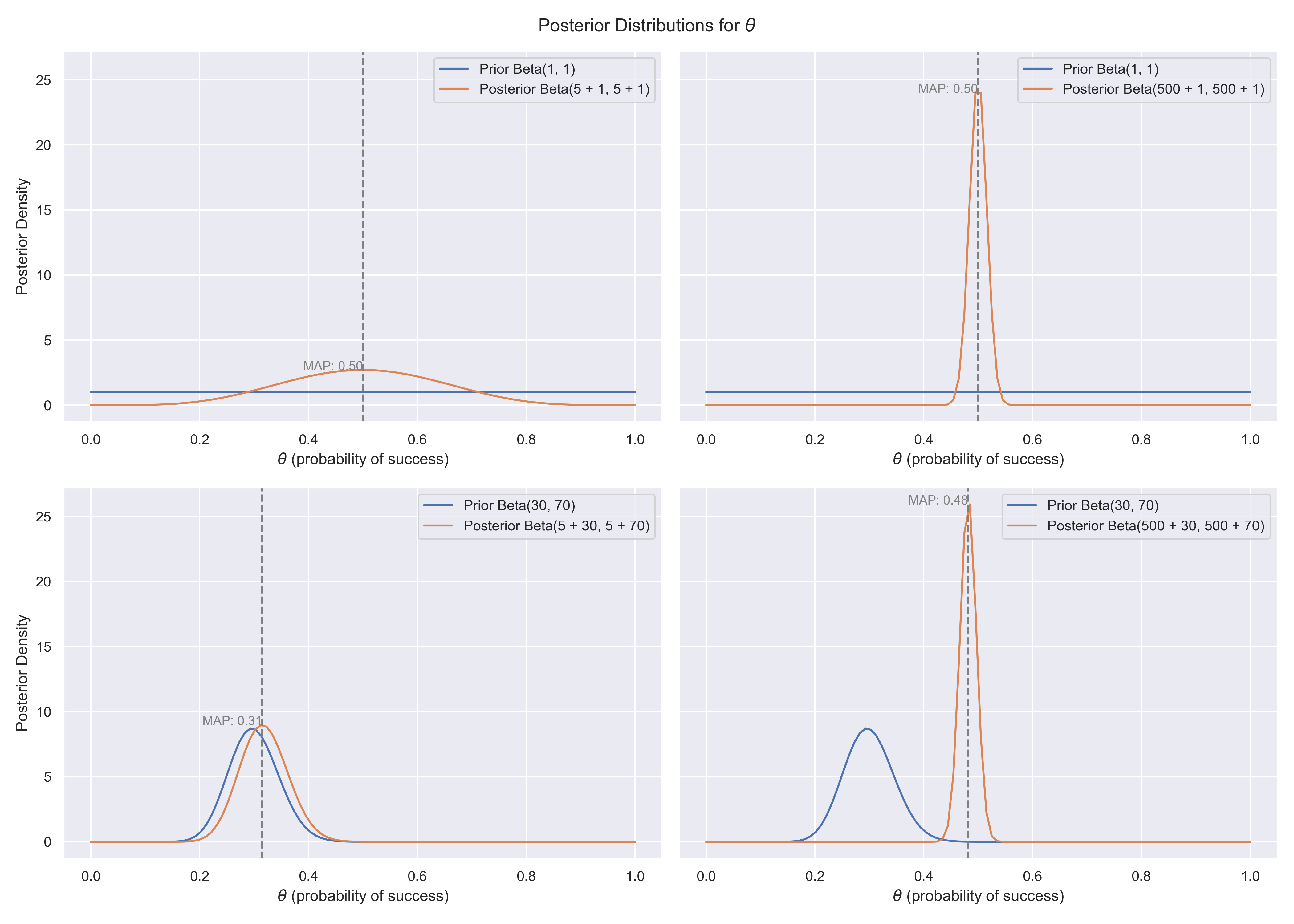
The choice of $\alpha$ and $\beta$ depends on our prior belief about the distribution of $\theta$. If we know very little, we can choose $\alpha = \beta = 1$ to obtain a uniform non-informative prior. Such a prior would assign equal probability to every possible value of $\theta$ (namely 1. If it seems odd that different values can have a probability of 1, remember that the probability distribution must integrate to 1).

If we have strong reason to believe that $\theta \approx 0.3$, e.g. because we have observed 300 successes in 1000 trials, then it would be very reasonable to set $\alpha = 300$ and $\beta = 700$ (note that $\alpha$ is equal to the expected number of successes, and $\beta$ is the expected number of failures). With a stronger prior, like that one, the posterior distribution will be similar to the prior, unless observed data strongly contradicts this. For a non-informative prior, such as the uniform prior, the data will have a bigger impact on the posterior initially. However, with sufficient data, the posterior will eventually converge to the true value of $\theta$ regardless of the choice of prior.