Neural Networks: How Backpropagation Works
30 October 2025The world probably doesn’t need another this-is-how-neural-networks-work article, but I don’t really feel like I know something until I have seen and worked through the formulas. This is the result of that.
I will assume you are already familiar with neural networks –maybe you know how to configure one in tensorflow or pytorch, because I’m not going to go into detail about what layers, nodes and activation functions are. There are plenty materials online for that. I will specifically focus on the formulas of back-propagation.
So let’s set the scene:

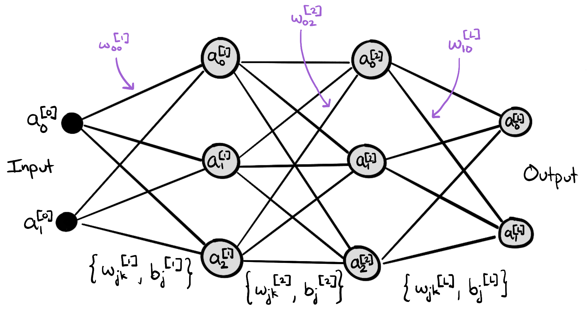
We will let $a_j^{[l]}$ denote the output of node $j$ in layer $l$. So $a_0^{[1]}$ is the output of the first (index 0) node in layer 1, and $a_4^{[3]}$ for the output of the 3rd node in layer 3, etc.
$a_j^{[0]}$ is the input data ($l=0$). That’s the starting point.
Then we take the weighted average of the inputs with bias:
\[\begin{equation} z_{j}^{[l]} = \sum_k w_{jk}^{[l]}a_k^{[l-1]} + b_j^{[l]} \end{equation}\]Note on notation: $w_{jk}^{[l]}$ is the weight from node $k$ in layer $l-1$ to node $j$ in layer $l.$ It’s intuitive to read it from left to right as “weight from node $j$ to node $k$”, but that’s not the convention and mathematics is nothing if not conventional. So I will stick with convention.
The weights $w$ and biases $b$ are initialized, which roughly means they are randomly chosen in the beginning.
We apply an activation function $\sigma$ and let that be the output of the node $j$:
\[\begin{equation} a_j^{[l]} = \sigma(z_j^{[l]}) = \sigma(\sum_k w_{jk}^{[l]}a_k^{[l-1]} + b_j^{[l]}) \label{node} \end{equation}\]Another note on notation: $\sigma$ could be different for each layer, but we don’t need to assume a specific functional form for backpropagation to work, so I will just write $\sigma$ for simplicity instead of the more accurate $\sigma_l$ or $\sigma^{[l]}$.
One forward pass through the network calculates all activations/outputs and the cost (average loss) $\mathcal{C}$. The point is to minimize the cost. So “training” the network means finding weights and biases that minimize the cost function. We do this in steps by incrementally updating the weights and biases in such a way that it will result in a lower cost.
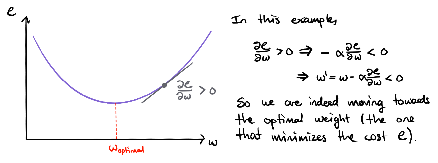
The idea is simple: we evaluate how the cost $\mathcal{C}$ will change w.r.t to the weight $w_{jk}^{[l]}$ and bias $b_j^{[l]}$ and update them accordingly like this:
\[\begin{gather} w^{\prime}= w-\alpha \frac{\partial \mathcal{C}}{\partial w} \\ b^{\prime}= b-\alpha \frac{\partial \mathcal{C}}{\partial b} \end{gather}\](yes, I am butchering the notation by dropping the sub- and superscripts, but they make the equations unnecessarily difficult-looking. Don’t worry, I will bring them back in a sec.)
$\alpha$ is the step size or learning rate that is defined before training the network (and can be tuned). While the gradient tells us which direction to go, $\alpha$ tells us how many steps to take.

The goal of propagation is to do these calculations efficiently for every weight and bias for arbitrary deep neural networks. The key to achieving this is the chain rule for derivatives.
First, we consider the auxiliary gradient $\delta_j^{[l]} := \frac{\partial \mathcal{C}}{\partial z_j^{[l]}}$, which will make everything that follows easier. $\mathcal{C}$ is a function of all the outputs $a_j^{[l]}$, and each output $a_j^{[l]}$ is a function of $z_j^{[l]}$, so we can apply the chain rule:
\[\begin{equation} \delta_j^{[l]} := \frac{\partial \mathcal{C}}{\partial z_j^{[l]}} = \sum_k \frac{\partial \mathcal{C}}{\partial a_k^{[l]}} \frac{\partial a_k^{[l]}}{\partial z_j^{[l]}}. \end{equation}\]We can get rid of the summation by considering what happens to $\tfrac{\partial a_k^{[l]}}{\partial z_j^{[l]}}$ when $k \neq j$; $a_k^{[l]}$ only depends on $z_j^{[l]}$ if $k = j$ (refer back to \eqref{node}), so $\tfrac{\partial a_k}{\partial z_j}=0$ for $k \neq j$. Hence, all terms, except for one, vanish:
\[\begin{align} \delta_j^{[l]} &= \frac{\partial \mathcal{C}}{\partial a_j^{[l]}} \frac{\partial a_j^{[l]}}{\partial z_j} \\ &= \frac{\partial \mathcal{C}}{\partial a_j^{[l]}} \sigma^{\prime}(z_j^{[l]}) \label{delta-L} \end{align}\]That’s one application of the chain rule. Now we will apply it differently, by noting that $z_j^{[l]}$ is a function of $z_j^{[l+1]}$, so we can write
\[\delta_j^{[l]} = \sum_k \frac{\partial \mathcal{C}}{\partial z_k^{[l+1]}} \frac{\partial z_k^{[l+1]}}{\partial z_j^{[l]}}.\]Let’s see if we can do something to $\frac{\partial z_k^{[l+1]}}{\partial z_j^{[l]}}$. Since \(\begin{align} z_k^{[l+1]} &= \sum_j w_{kj}^{[l+1]}a_j^{[l]}+b_k^{[l+1]}\\&=\sum_j w_{kj}^{[l+1]}\sigma(z_j^{[l]})+b_k^{[l+1]}, \end{align}\)
we can write
\[\begin{equation} \frac{\partial z_k^{[l+1]}}{\partial z_j^{[l]}} = w_{kj}^{[l+1]}\sigma^{\prime}(z_j^{[l]}). \end{equation}\]Similar to earlier, most of the terms in the sum become 0 when we differentiate w.r.t $z_j^{[l]}$.
Hence,
\[\begin{align} \delta_j^{[l]} &= \sum_k \frac{\partial \mathcal{C}}{\partial z_k^{[l+1]}}w_{kj}^{[l+1]}\sigma^{\prime}(z_j^{[l]}) \\ &=\sum_k \delta_{k}^{[l+1]}w_{kj}^{[l+1]}\sigma^{\prime}(z_j^{[l]})\label{delta_l}. \end{align}\]Now we have done most of the hard work and can finally consider $\frac{\partial \mathcal{C}}{\partial b_j^{[l]}}$ and $\frac{\partial \mathcal{C}}{\partial w_{jk}^{[l]}}$ by applying (you guessed it) the chain rule:
\[\begin{align} \frac{\partial \mathcal{C}}{\partial b_j^{[l]}} &= \sum_k \frac{\partial \mathcal{C}}{\partial z_k^{[l]}} \underbrace{\frac{\partial z_k^{[l]}}{\partial b_j^{[l]}}}_{=1} \\ &= \sum_k \frac{\partial \mathcal{C}}{\partial z_k^{[l]}} \\ &= \frac{\partial \mathcal{C}}{\partial z_j^{[l]}} \\ &= \delta_j^{[l]}, \end{align}\]and
\[\begin{align} \frac{\partial \mathcal{C}}{\partial w_{jk}^{[l]}} &= \frac{\partial \mathcal{C}}{\partial z_j^{[l]}} \underbrace{\frac{\partial z_j^{[l]}}{\partial w_{jk}^{[l]}}}_{= a_k^{[l-1]}} \\ &= \frac{\partial \mathcal{C}}{\partial z_j^{[l]}}a_k^{[l-1]} \\ &= \delta_j^{[l]} a_k^{[l-1]}. \end{align}\]Now we have everything in place to calculate the gradients efficiently because we don’t need to compute gradients directly at every layer. For the output layer we will use equation \eqref{delta-L}, so we need to compute $\tfrac{\partial \mathcal{C}}{\partial a_j^{[L]}}$ and $\sigma^{\prime} (z_j^{[L]})$. They depend on our choices of cost function and activation function, but we usually choose those so that the derivate is easy to obtain. For example, if we choose (half) squared error as our cost, then $\frac{\partial \mathcal{C}}{\partial a_j^{[L]}}$ is simply $a_j-y_j$. Similarly, if the activation function is the identity function, then the derivative is just $z_j^{[L]}$. Easy!
For the earlier layers, we don’t need to compute the gradient of the cost directly because we can just use equation \eqref{delta_l} whose terms we have already computed. And that’s how it goes all the way from the last layer to the first. So to summarize, the equations needed for backpropagation are:
\[\begin{align} \delta_j^{[L]} &= \frac{\partial \mathcal{C}}{\partial a_j} \sigma^{\prime}(z_j) \\ \delta_j^{[l]} &= \sum_k \delta_{k}^{[l+1]}w_{kj}^{[l+1]}\sigma^{\prime}(z_j^{[l]}) \\ \frac{\partial \mathcal{C}}{\partial b_j^{[l]}} &= \delta_j^{[l]} \\ \frac{\partial \mathcal{C}}{\partial w_{jk}^{[l]}} &= \delta_j^{[l]} a_k^{[l-1]}, \end{align}\]References
- Victor E. Bazterra, Xmas blog: Andrew Ng’s missing notes about back-propagation
- Michael A. Nielsen, “Neural Networks and Deep Learning”, chapter 2, Determination Press, 2015